Our World in Data Examples

Data sets

This work references data on life expectancy and causes of death from the Our World In Data organization. The life expectancy and survival rate graphics reference the specific section of the site here. The causes of death graphics reference the specific section of the site here.

life_expectancy_data <- tibble(read.csv("docs/life-expectancy.csv")) %>%
  arrange(Entity, Year)
colnames(life_expectancy_data) <- c("Entity", "Code", "Year", "Expectancy")

men_survival_to_age_65 <- tibble(read.csv("docs/men-survival-to-age-65.csv")) %>%
  arrange(Entity, Year)
colnames(men_survival_to_age_65) <- c("Entity", "Code", "Year", "Percent")

women_survival_to_age_65 <- tibble(read.csv("docs/women-survival-to-age-65.csv")) %>%
  arrange(Entity, Year)
colnames(women_survival_to_age_65) <- c("Entity", "Code", "Year", "Percent")

causes <- c("Executions", "Meningitis", "Lower_Respiratory_Infections",
            "Intestinal_Infectious_Diseases", "Protein-Energy_Malnutrition", "Terrorism",
            "Cardiovascular_Diseases", "Dementias", "Kidney_Disease", 
            "Respiratory_Diseases", "Liver_Diseases", "Digestive_Diseases", 
            "Hepatitis", "Cancers", "Parkinson_Disease", "Fire", "Malaria", "Drowning", 
            "Homicide", "HIV/AIDS", "Drug_Use_Disorders", "Tuberculosis", 
            "Road_Injuries", "Maternal_Disorders", "Neonatal_Disorders", "Alcohol_Use_Disorders",
            "Natural_Disasters", "Diarrheal_Diseases", "Heat_And_Cold_Exposure", 
            "Nutritional_Deficiencies", "Suicide", "Conflict", "Diabetes", "Poisonings")

causes_of_death <- tibble(read.csv("docs/annual-number-of-deaths-by-cause.csv")) %>%
  arrange(Entity, Year)
colnames(causes_of_death) <- c("Entity", "Code", "Year", all_of(causes))
causes_of_death <- causes_of_death %>% mutate(Executions = as.numeric(Executions))

Plotting functions

The code snippet here shows the plotting designs used in following graphics tabs.

# various plot designs used in the analysis

le_plot_single <- function(data) {
  ggplot(data, aes(Year, Expectancy)) +
    geom_line() +
    labs(
      x = "Year",
      y = "Life Expectancy",
      title = "Life expectancy",
      subtitle = "1770 to 2019",
      caption = "Source: Our World In Data"
    ) +
    theme_minimal() +
    scale_y_continuous(limits = c(20, 90), breaks = seq(20, 90, by = 10)) +
    theme(legend.position = "none") +
    scale_colour_brewer(palette = "Dark2")
}

le_plot_multi <- function(data, color_lab) {
  ggplot(data, aes(Year, Expectancy, color = Entity)) +
    geom_line() +
    labs(
      x = "Year",
      y = "Life Expectancy",
      title = "Life expectancy",
      color = color_lab,
      subtitle = "1770 to 2019",
      caption = "Source: Our World In Data"
    ) +
    theme_minimal() +
    scale_y_continuous(limits = c(20, 90), breaks = seq(20, 90, by = 10)) +
    theme(legend.position = "bottom") +
    scale_colour_brewer(palette = "Dark2")
}

sr_plot <- function(data, title_lab, color_lab) {
  ggplot(data, aes(Year, Percent, color = Entity)) +
    geom_line() +
    labs(title = title_lab,
         color = color_lab) +
    theme_minimal() +
    scale_y_continuous(limits = c(20, 100),
                       breaks = seq(20, 100, by = 10)) +
    scale_colour_brewer(palette = "Dark2")
}

cod_plot <- function(data, xlab, end_scale, increment) {
  ggplot(data, aes(Count, Cause)) +
    geom_col(aes(fill = Count)) +
    theme_minimal() +
    theme(legend.position = 'none') +
    scale_fill_distiller(palette = "Dark2") +
    geom_label(
      aes(label = Count),
      size = 3,
      hjust = -0.1,
      label.size = 0.1,
      label.padding = unit(0.1, "lines")
    ) +
    scale_x_continuous(limits = c(0, end_scale), breaks = seq(0, end_scale, by = increment)) +
    labs(x = xlab,
         y = "")
}

Life Expectancy

These graphs show period life expectancy at birth: the average number of years a newborn would live if the pattern of mortality in the given year were to stay the same throughout its life.

The World

life_expectancy_data %>%
  filter(Entity == "World") %>%
  le_plot_single()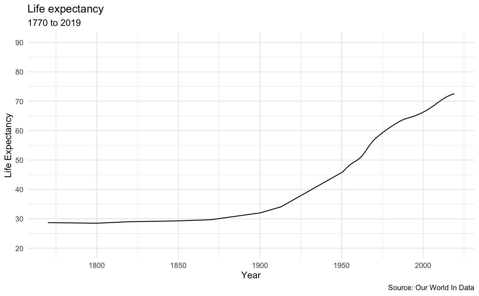

Regions

sample_list <- c("Oceania", "Europe", "Americas", "Asia", "Africa", "World")

life_expectancy_data %>%
  filter(Entity %in% sample_list) %>%
  le_plot_multi("Region")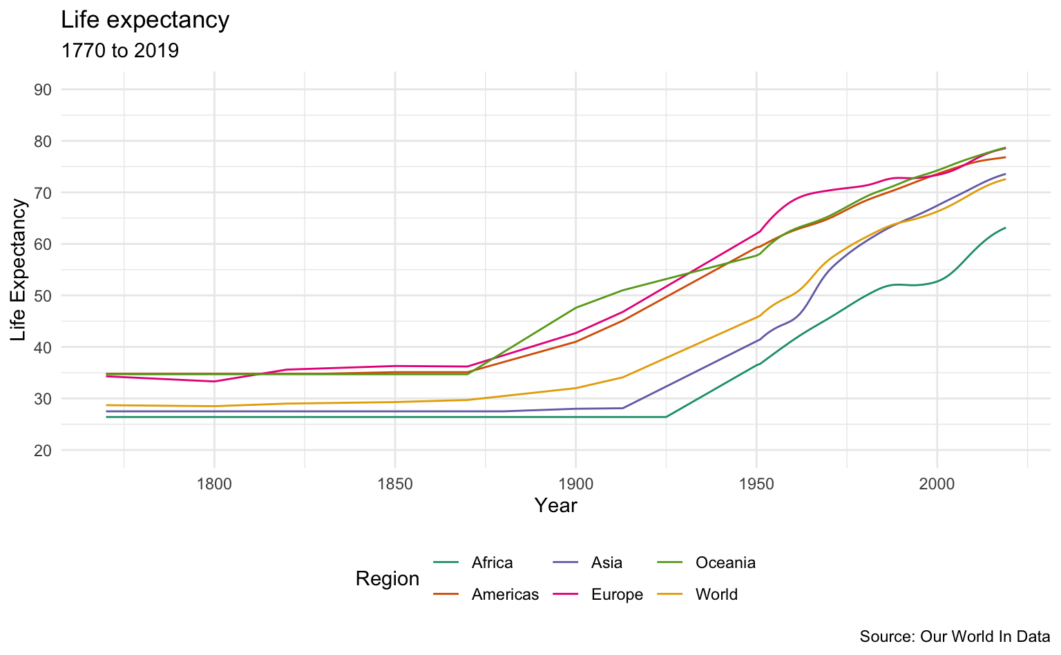

Selected Countries

sample_list <- c("Japan", "South Korea", "United Kingdom", "India", "Ethiopia", "South Africa", "United States", "World")

life_expectancy_data %>%
  filter(Entity %in% sample_list) %>%
  filter(Year >= 1865) %>%
  le_plot_multi("Country")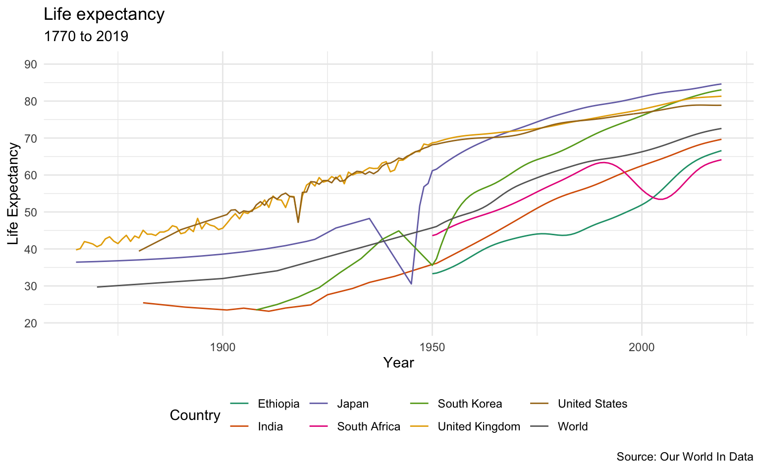

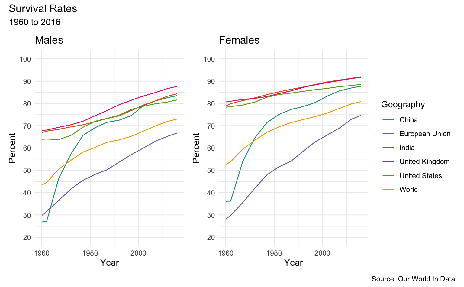
Survival Rates

These graphs show the share of the population that is expected to survive to the age of 65.

Selected Geographies

sample_list <- c("United States", "China", "Philipines", "United Kingdom", "European Union", "India", "World")

m <- men_survival_to_age_65 %>%
  filter(Entity %in% sample_list) %>%
  sr_plot("Males", "Geography")

w <- women_survival_to_age_65 %>%
  filter(Entity %in% sample_list) %>%
  sr_plot("Females", "Geography")

m + w + plot_layout(ncol = 2, guides = "collect") + 
  plot_annotation(
    title = "Survival Rates",
    subtitle = "1960 to 2016",
    caption = "Source: Our World In Data"
  )

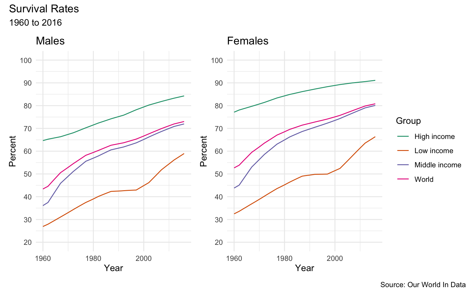
By Income Distribution Group World-wide

sample_list <- c("High income", "Middle income", "Low income", "World")

m <- men_survival_to_age_65 %>%
  filter(Entity %in% sample_list) %>%
  sr_plot("Males", "Group")

w <- women_survival_to_age_65 %>%
  filter(Entity %in% sample_list) %>%
  sr_plot("Females", "Group")

m + w + plot_layout(ncol = 2, guides = "collect") + 
  plot_annotation(
    title = "Survival Rates",
    subtitle = "1960 to 2016",
    caption = "Source: Our World In Data"
  )

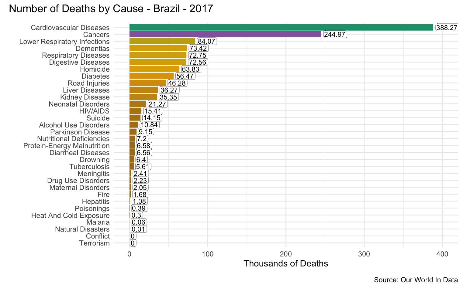
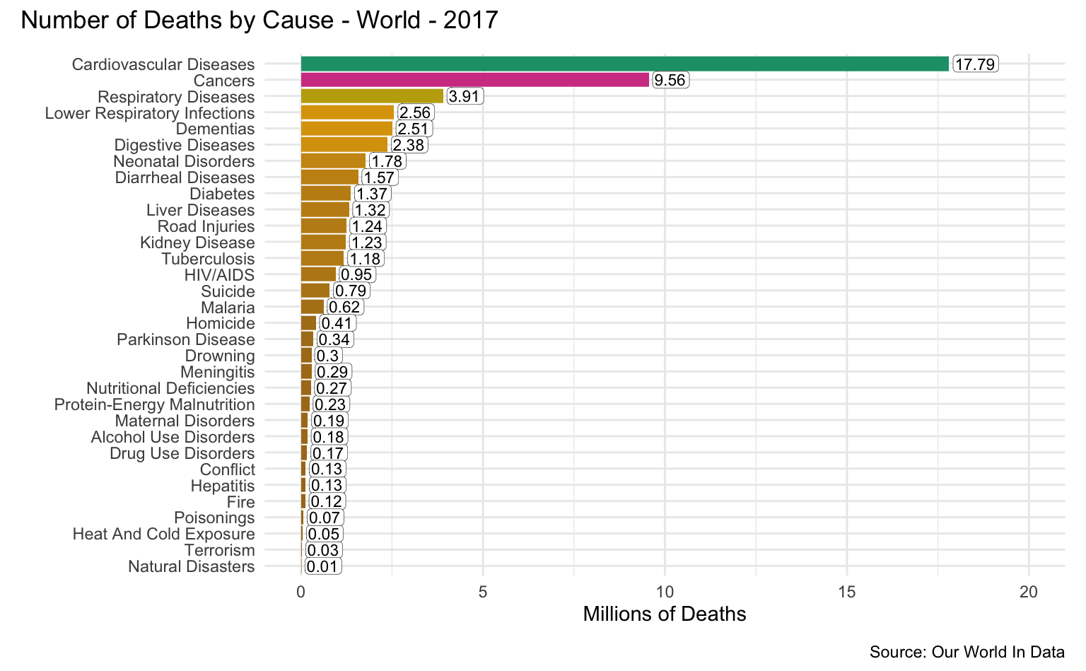
Causes of Death

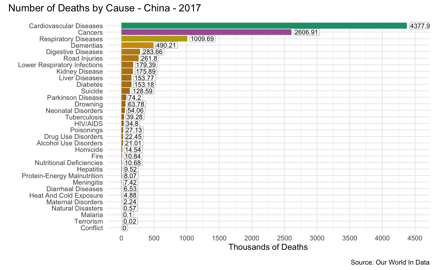
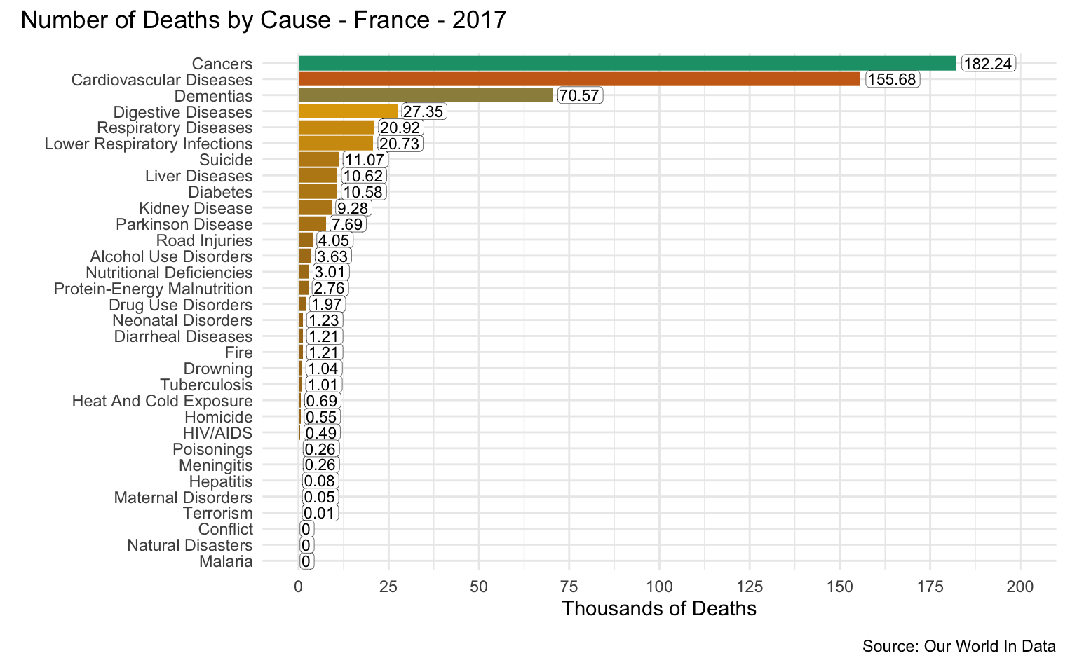
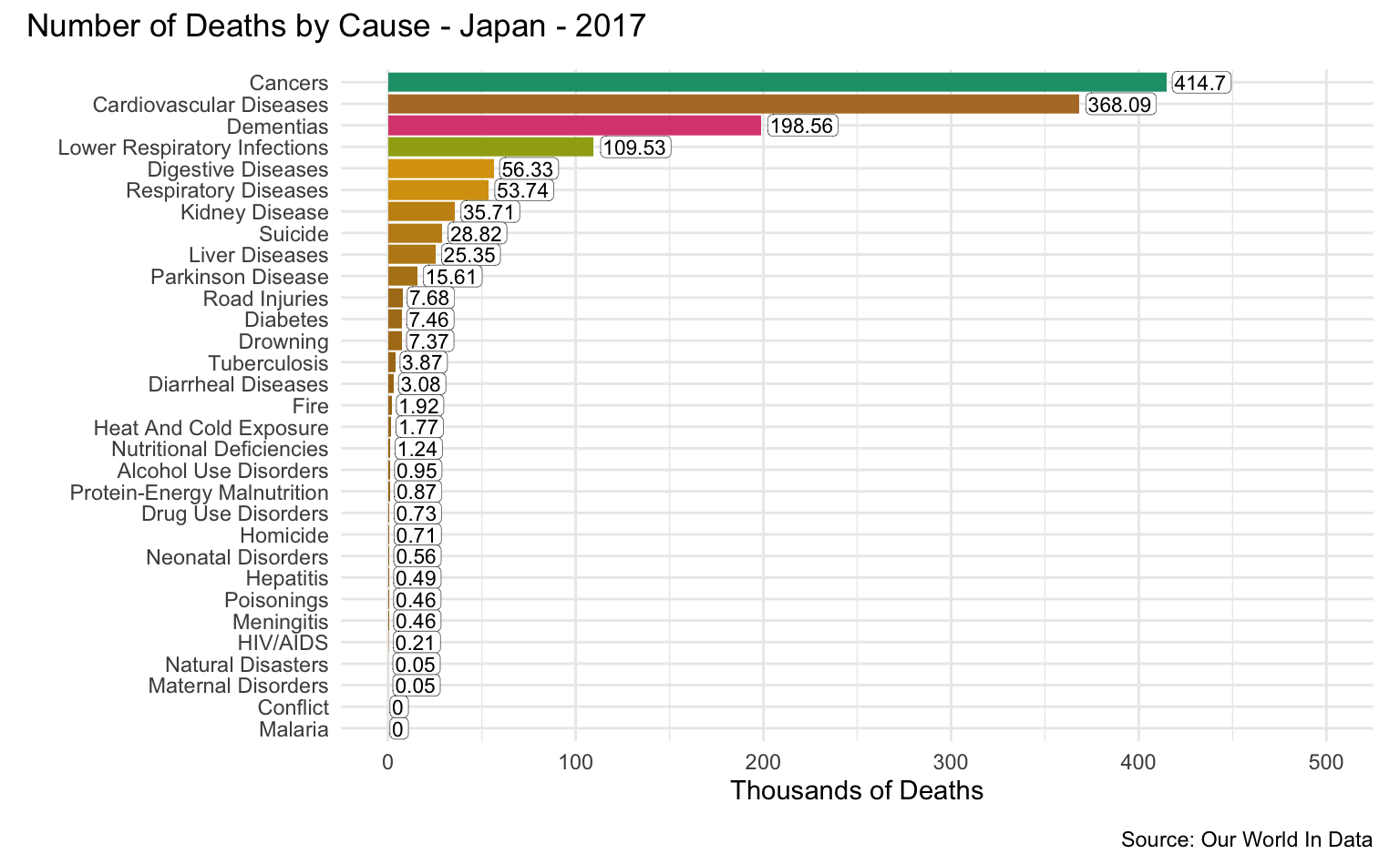
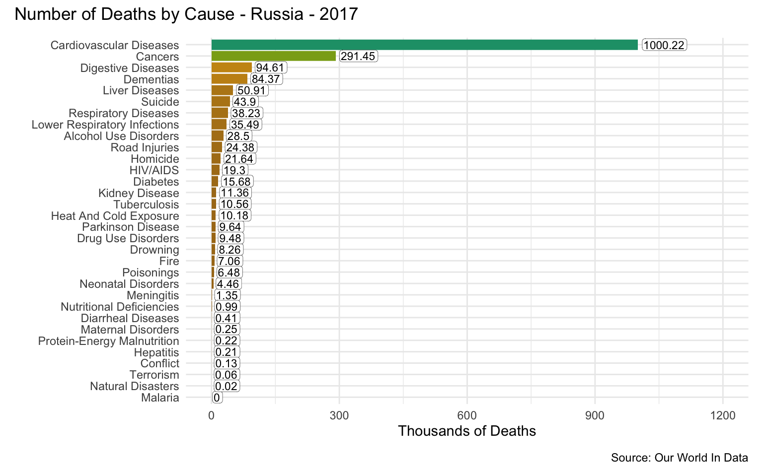
The Global Burden of Disease is a major global study on the causes of death and disease published in the medical journal The Lancet. These estimates of the annual number of deaths by cause are shown in these graphics.

World

latest_year <- max(causes_of_death$Year)

g <- causes_of_death %>%
  filter(Entity == "World") %>%
  filter(Year == latest_year) %>%
  pivot_longer(all_of(causes), names_to = "Cause", values_to = "Count") %>%
  filter(!is.na(Count)) %>% 
  mutate(
    Count = round(Count / 1000000, 2),
    Cause = reorder(as_factor(str_replace_all(Cause, "_", " ")), Count)
  ) %>% 
  cod_plot("Millions of Deaths", 20, 5)

g + plot_annotation(
  title = str_c("Number of Deaths by Cause - World - ", latest_year),
  caption = "Source: Our World In Data"
)

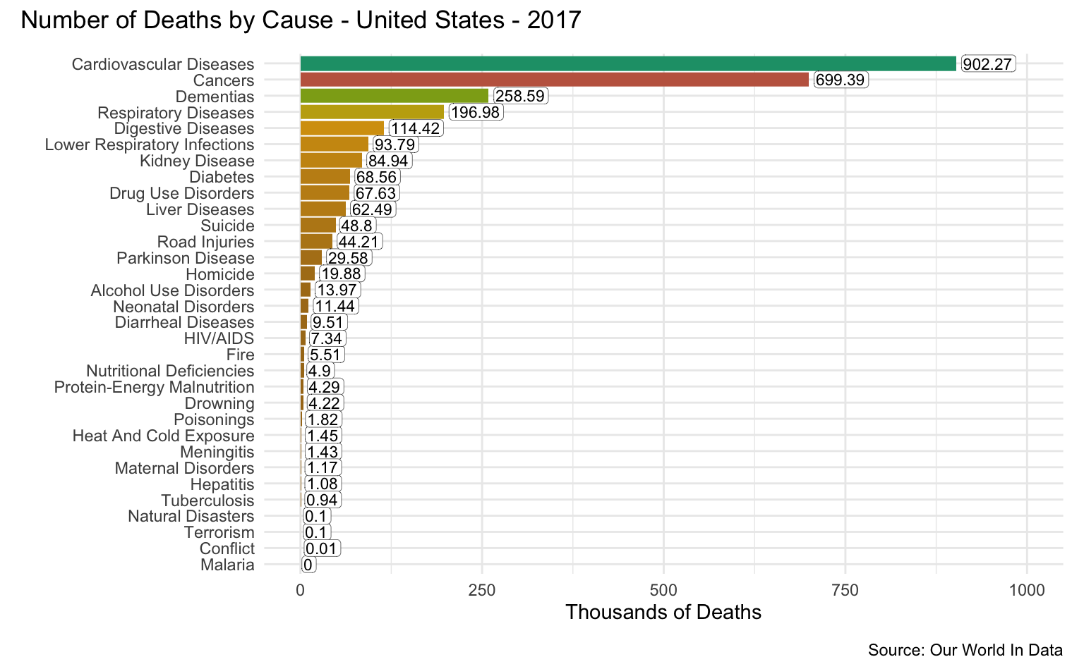
United States

latest_year <- max(causes_of_death$Year)

g <- causes_of_death %>%
  filter(Entity == "United States") %>%
  filter(Year == latest_year) %>%
  pivot_longer(all_of(causes), names_to = "Cause", values_to = "Count") %>%
  filter(!is.na(Count)) %>% 
  mutate(
    Count = round(Count / 1000, 2),
    Cause = reorder(as_factor(str_replace_all(Cause, "_", " ")), Count)
  ) %>% 
  cod_plot("Thousands of Deaths", 1000, 250)

g + plot_annotation(
  title = str_c("Number of Deaths by Cause - United States - ", latest_year),
  caption = "Source: Our World In Data"
)

China

latest_year <- max(causes_of_death$Year)

g <- causes_of_death %>%
  filter(Entity == "China") %>%
  filter(Year == latest_year) %>%
  pivot_longer(all_of(causes), names_to = "Cause", values_to = "Count") %>%
  filter(!is.na(Count)) %>% 
  mutate(
    Count = round(Count / 1000, 2),
    Cause = reorder(as_factor(str_replace_all(Cause, "_", " ")), Count)
  ) %>% 
  cod_plot("Thousands of Deaths", 4500, 500)

g + plot_annotation(
  title = str_c("Number of Deaths by Cause - China - ", latest_year),
  caption = "Source: Our World In Data"
)

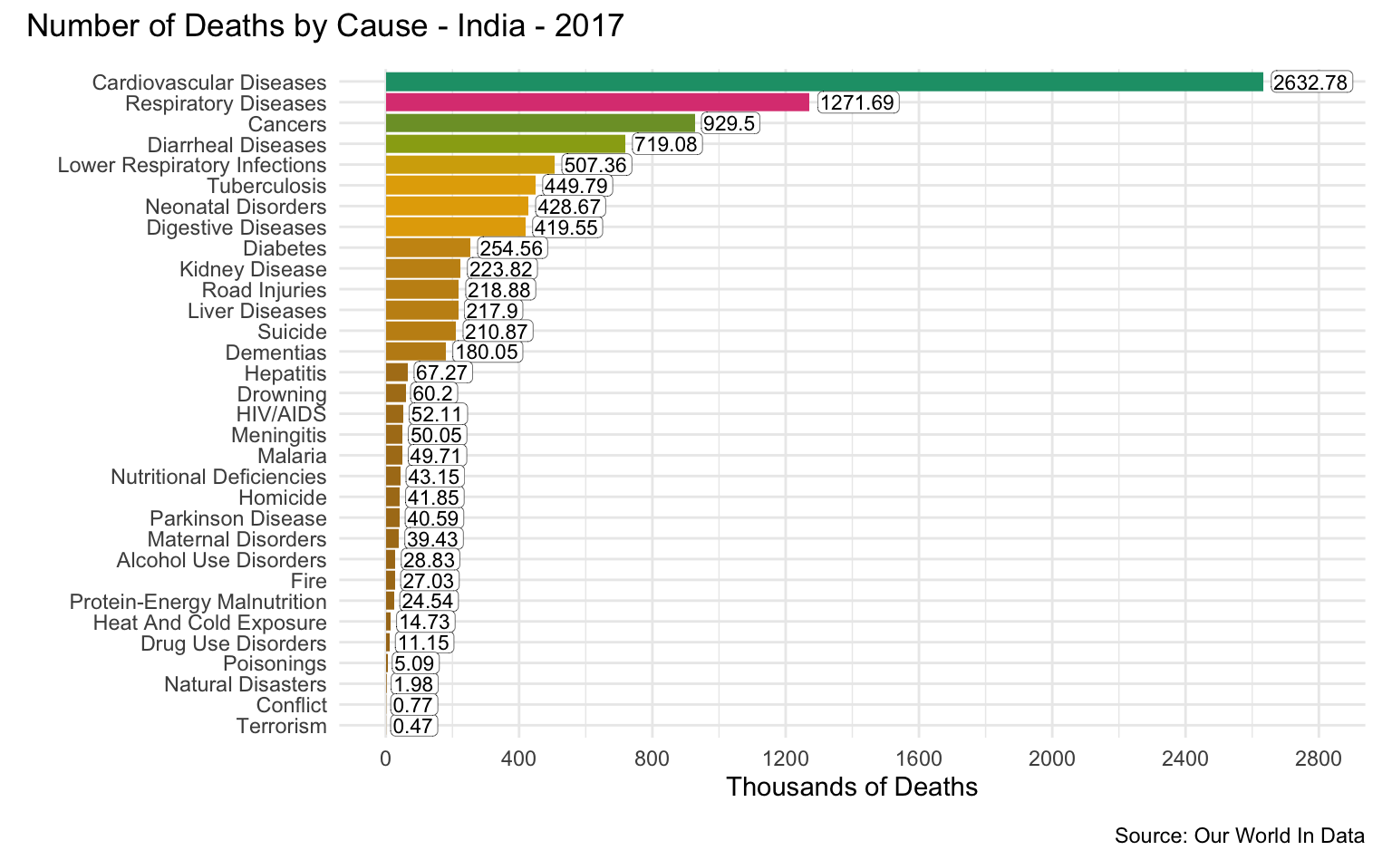
India

latest_year <- max(causes_of_death$Year)

g <- causes_of_death %>%
  filter(Entity == "India") %>%
  filter(Year == latest_year) %>%
  pivot_longer(all_of(causes), names_to = "Cause", values_to = "Count") %>%
  filter(!is.na(Count)) %>% 
  mutate(
    Count = round(Count / 1000, 2),
    Cause = reorder(as_factor(str_replace_all(Cause, "_", " ")), Count)
  ) %>% 
  cod_plot("Thousands of Deaths", 2800, 400)

g + plot_annotation(
  title = str_c("Number of Deaths by Cause - India - ", latest_year),
  caption = "Source: Our World In Data"
)

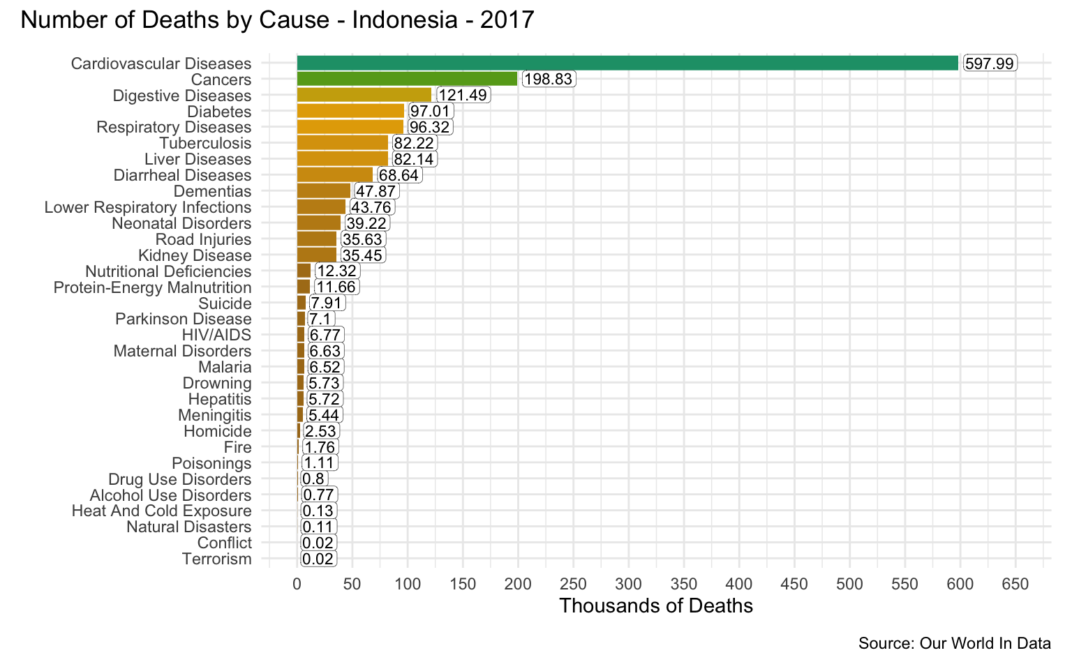
Indonesia

latest_year <- max(causes_of_death$Year)

g <- causes_of_death %>%
  filter(Entity == "Indonesia") %>%
  filter(Year == latest_year) %>%
  pivot_longer(all_of(causes), names_to = "Cause", values_to = "Count") %>%
  filter(!is.na(Count)) %>% 
  mutate(
    Count = round(Count / 1000, 2),
    Cause = reorder(as_factor(str_replace_all(Cause, "_", " ")), Count)
  ) %>% 
  cod_plot("Thousands of Deaths", 650, 50)

g + plot_annotation(
  title = str_c("Number of Deaths by Cause - Indonesia - ", latest_year),
  caption = "Source: Our World In Data"
)

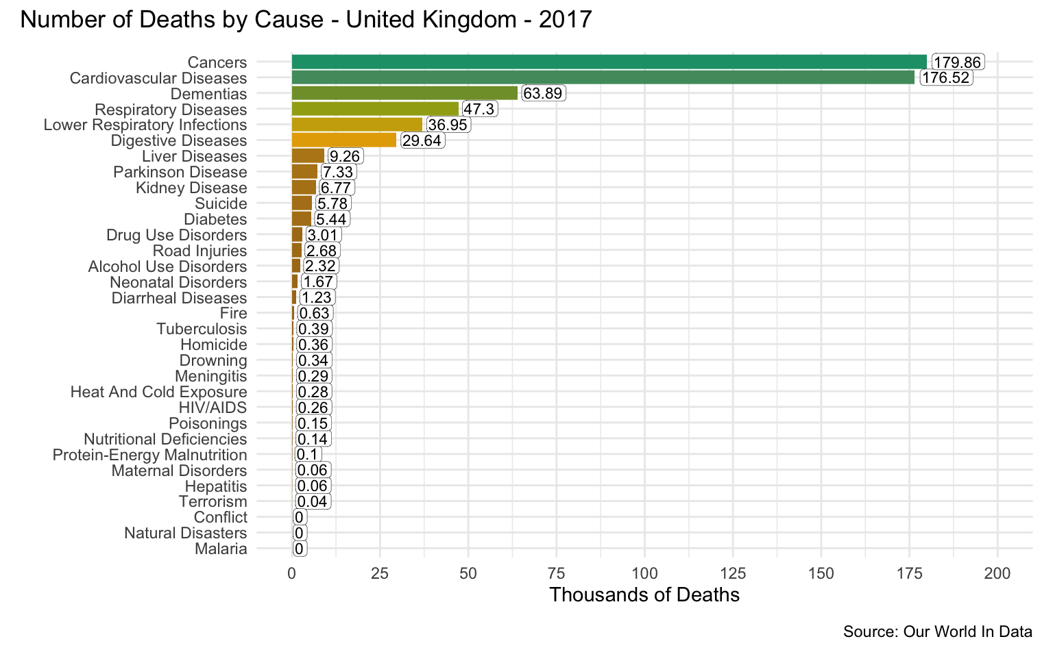
United Kingdom

latest_year <- max(causes_of_death$Year)

g <- causes_of_death %>%
  filter(Entity == "United Kingdom") %>%
  filter(Year == latest_year) %>%
  pivot_longer(all_of(causes), names_to = "Cause", values_to = "Count") %>%
  filter(!is.na(Count)) %>% 
  mutate(
    Count = round(Count / 1000, 2),
    Cause = reorder(as_factor(str_replace_all(Cause, "_", " ")), Count)
  ) %>% 
  cod_plot("Thousands of Deaths", 200, 25)

g + plot_annotation(
  title = str_c("Number of Deaths by Cause - United Kingdom - ", latest_year),
  caption = "Source: Our World In Data"
)

France

latest_year <- max(causes_of_death$Year)

g <- causes_of_death %>%
  filter(Entity == "France") %>%
  filter(Year == latest_year) %>%
  pivot_longer(all_of(causes), names_to = "Cause", values_to = "Count") %>%
  filter(!is.na(Count)) %>% 
  mutate(
    Count = round(Count / 1000, 2),
    Cause = reorder(as_factor(str_replace_all(Cause, "_", " ")), Count)
  ) %>% 
  cod_plot("Thousands of Deaths", 200, 25)

g + plot_annotation(
  title = str_c("Number of Deaths by Cause - France - ", latest_year),
  caption = "Source: Our World In Data"
)

Japan

latest_year <- max(causes_of_death$Year)

g <- causes_of_death %>%
  filter(Entity == "Japan") %>%
  filter(Year == latest_year) %>%
  pivot_longer(all_of(causes), names_to = "Cause", values_to = "Count") %>%
  filter(!is.na(Count)) %>% 
  mutate(
    Count = round(Count / 1000, 2),
    Cause = reorder(as_factor(str_replace_all(Cause, "_", " ")), Count)
  ) %>% 
  cod_plot("Thousands of Deaths", 500, 100)

g + plot_annotation(
  title = str_c("Number of Deaths by Cause - Japan - ", latest_year),
  caption = "Source: Our World In Data"
)

Russia

latest_year <- max(causes_of_death$Year)

g <- causes_of_death %>%
  filter(Entity == "Russia") %>%
  filter(Year == latest_year) %>%
  pivot_longer(all_of(causes), names_to = "Cause", values_to = "Count") %>%
  filter(!is.na(Count)) %>% 
  mutate(
    Count = round(Count / 1000, 2),
    Cause = reorder(as_factor(str_replace_all(Cause, "_", " ")), Count)
  ) %>% 
  cod_plot("Thousands of Deaths", 1200, 300)

g + plot_annotation(
  title = str_c("Number of Deaths by Cause - Russia - ", latest_year),
  caption = "Source: Our World In Data"
)

Brazil

latest_year <- max(causes_of_death$Year)

g <- causes_of_death %>%
  filter(Entity == "Brazil") %>%
  filter(Year == latest_year) %>%
  pivot_longer(all_of(causes), names_to = "Cause", values_to = "Count") %>%
  filter(!is.na(Count)) %>% 
  mutate(
    Count = round(Count / 1000, 2),
    Cause = reorder(as_factor(str_replace_all(Cause, "_", " ")), Count)
  ) %>% 
  cod_plot("Thousands of Deaths", 400, 100)

g + plot_annotation(
  title = str_c("Number of Deaths by Cause - Brazil - ", latest_year),
  caption = "Source: Our World In Data"
)